How to R - Beginner Guide Time Series Analysis
- Data Science
- beginners guide, forecast, r, time series
- 5 min reading time

Dr. Stefan Lieder

In the tutorial "How to R - Beginner Guide Time Series Analysis", a time series analysis with R is carried out, outlining the essential steps of data preparation, modelling and visualization. The focus is on the use of the R packages tidyverse, tsibble and fable.
Table of contents
Time series analysis with R
In this short tutorial, we will limit ourselves to briefly outlining the essential steps in time series analysis in the R programming language.
These are:
- Data preparation,
- Modeling and
- Visualization.
We use the R packages tidyverse, tsibble and fable for this.
Data preparation
As a rule, all necessary functions for general data preparation are contained in the "tidyverse" package collection. For data preparation in the "tidy" style, however, the "tsibble" package is also needed. First we load the packages and the data:
					library(fable)

library(tsibble)
library(tidyverse, quietly = TRUE, warn.conflicts = FALSE)

raw_data  = read_delim("~/Documents/Progonosewerkstatt/Peer_Labs/R/2_DataPreparation/01_Data/Company.csv", delim=";")

glimpse(raw_data)

## Rows: 101
## Columns: 9
## $ Month       <dttm> 2011-01-01, 2011-02-01, 2011-03-01, 2011-04-01, 2011-05-…
## $ Germany     <dbl> 19722000, 25062000, 47066000, 52625000, 66489000, 5660100…
## $ Canada      <dbl> 1809000, 2206000, 3035000, 3793000, 4813000, 4370000, 454…
## $ Switzerland <dbl> 3624000, 4972000, 7010000, 7084000, 9452000, 7971000, 733…
## $ Austria     <dbl> 1436000, 2390000, 6556000, 7544000, 9069000, 8154000, 817…
## $ US          <dbl> 3598000, 3349000, 6101000, 6098000, 6935000, 8644000, 757…
## $ France      <dbl> 4861000, 5465000, 8440000, 8223000, 9706000, 8809000, 806…
## $ Sweden      <dbl> 10723000, 12333000, 23562000, 30595000, 46253000, 3886900…
## $ China       <dbl> 8103000, 4040000, 25974000, 34776000, 31125000, 31576000,…


Im “tidy”-Style werden die Daten im Long-Format benötigt. Wir nutzen die “pivot_longer” Funktion. Anschliessend konvertieren wir das tibble-Objekt (= tidy dataframe) in ein tsibble Objekt, welches ein dataframe für Zeitreihen ist.

prep_data = raw_data %>%
  pivot_longer(., cols = 2:9, names_to = "Subsidiary", values_to = "Revenues") %>%
  mutate(Month = yearmonth(Month)) %>%
  tsibble(., key = Subsidiary, index = Month)
glimpse(prep_data)

## Rows: 808
## Columns: 3
## Key: Subsidiary [8]
## $ Month      <mth> 2011 Jan, 2011 Feb, 2011 Mar, 2011 Apr, 2011 May, 2011 Jun…
## $ Subsidiary <chr> "Austria", "Austria", "Austria", "Austria", "Austria", "Au…
## $ Revenues   <dbl> 1436000, 2390000, 6556000, 7544000, 9069000, 8154000, 8173…
To get a feel for the data, let's look at it first.
prep_data %>% autoplot(Revenues)

We see that there is a break in the data between 2016 and early 2020. After consulting with the technical expert, we know that it is a system change and all values must be non-negative. We correct this.
					prep_data = prep_data %>%
  mutate(Revenues = abs(Revenues))
prep_data %>% autoplot(Revenues)
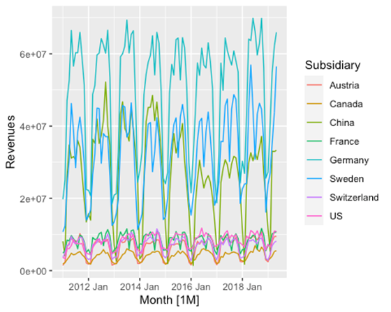
It can now be seen that the available time series have a strong seasonal character. The data are thus prepared and can be modelled.
Modelling the time series analysis
Two widely used models available in the Fable package are ETS and ARIMA. These models are specified with a compact formula representation. The response variable (Revenues) and all transformations are included on the left-hand side, while the model specification is on the right-hand side of the formula. If a model is not fully specified (or if the right-hand side of the formula is completely missing), the non-specified components are automatically selected.
We use both model classes to find the best model for the respective time series.
					fit <- prep_data %>%
  model(
    ets = ETS(Revenues),
    arima = ARIMA(Revenues)
  )
## Warning in sqrt(diag(best$var.coef)): NaNs produced
With coef() one can access all fit parameters of a model.
					fit %>% coef()
## # A tibble: 145 x 7
##    Subsidiary .model term  estimate std.error statistic p.value
##    <chr>      <chr>  <chr>    <dbl>     <dbl>     <dbl>   <dbl>
##  1 Austria    ets    alpha  2.21e-1        NA        NA      NA
##  2 Austria    ets    gamma  1.00e-4        NA        NA      NA
##  3 Austria    ets    l      6.43e+6        NA        NA      NA
##  4 Austria    ets    s0    -4.15e+6        NA        NA      NA
##  5 Austria    ets    s1    -3.35e+5        NA        NA      NA
##  6 Austria    ets    s2     2.47e+6        NA        NA      NA
##  7 Austria    ets    s3     2.42e+6        NA        NA      NA
##  8 Austria    ets    s4     1.35e+6        NA        NA      NA
##  9 Austria    ets    s5     1.78e+6        NA        NA      NA
## 10 Austria    ets    s6     1.82e+6        NA        NA      NA
## # … with 135 more rows
With glance, various statistical parameters of the fit of the model to the time series can be viewed.
					fit %>% glance
## # A tibble: 16 x 12
##    Subsidiary .model   sigma2 log_lik   AIC  AICc   BIC      MSE     AMSE
##    <chr>      <chr>     <dbl>   <dbl> <dbl> <dbl> <dbl>    <dbl>    <dbl>
##  1 Austria    ets    3.51e+11  -1568. 3166. 3172. 3205.  3.02e11  3.14e11
##  2 Canada     ets    1.08e- 2  -1529. 3088. 3093. 3127.  1.47e11  1.53e11
##  3 China      ets    1.84e+13  -1768. 3566. 3572. 3605.  1.59e13  2.76e13
##  4 France     ets    5.57e+11  -1591. 3213. 3218. 3252.  4.80e11  4.79e11
##  5 Germany    ets    1.98e+13  -1772. 3573. 3579. 3613.  1.71e13  1.73e13
##  6 Sweden     ets    1.08e+13  -1741. 3512. 3517. 3551.  9.26e12  1.02e13
##  7 Switzerla… ets    3.61e+11  -1569. 3169. 3175. 3208.  3.11e11  3.20e11
##  8 US         ets    5.81e- 3  -1568. 3172. 3181. 3219.  3.20e11  3.23e11
##  9 Austria    arima  4.55e+11  -1308. 2624. 2625. 2634. NA       NA
## 10 Canada     arima  1.82e+11  -1285. 2581. 2582. 2593. NA       NA
## 11 China      arima  2.07e+13  -1492. 2992. 2992. 3002. NA       NA
## 12 France     arima  5.13e+11  -1329. 2672. 2674. 2690. NA       NA
## 13 Germany    arima  2.20e+13  -1498. 3003. 3003. 3010. NA       NA
## 14 Sweden     arima  1.10e+13  -1468. 2944. 2944. 2954. NA       NA
## 15 Switzerla… arima  4.56e+11  -1322. 2655. 2655. 2667. NA       NA
## 16 US         arima  4.78e+11  -1311. 2633. 2634. 2648. NA       NA
## # … with 3 more variables: MAE <dbl>, ar_roots <list>, ma_roots <list>
With the forecast function we generate the forecasts for each time series from the models.
					fc = fit %>%
  forecast(h = "2 years")
Finally, we visualize the forecasts. It can be seen that both methods pick up the patterns of the individual time series and incorporate them into the forecast of their respective methodology, as is the case, for example, with the "summer slump" in the French subsidiary or the rising trend in the US company.
					fc %>% autoplot(prep_data) +
  ggtitle("Reveunes of Company's Subsidiaries")

Download Wiki article as a .pdf
Know more?
Would you like to delve deeper into this topic? Then we would be happy to talk to you personally about the areas of application of R - gladly also in connection with analytics products from SAP. Simply get in touch with us!

Published by:
Dr. Stefan Lieder
Former Head of Data Science Workshop
Dr. Stefan Lieder
How did you like the article?
How helpful was this post?
Click on a star to rate!
Average rating 0 / 5.
Number of ratings: 0
No votes so far! Be the first person to rate this post!


